Projecting three-point shooting for the 2022 draft class using hiearchical Bayesian modeling

A positive outlook for Ochai Agbaji, Jabari Smith, and Bennedict Mathurin

Three-point projection from college to the NBA is notoriously challenging — which makes attempting to predict it doubly interesting. One major challenge in this projection is the issue of small sample size: college players play at most 30 games per season and, with the exception of the best of the best, rarely take more than three or four threes per game.

This can produce artificially inflated or deflated shooting percentages more reflective of random noise than true player shooting skill. Bayesian shrinkage is one strategy for managing this randomness inherent in such a sparse dataset. I used a methodology heavily inspired by David Robinson’s series on empirical Bayesian estimation, and thank him for creating such an accessible and understandable introduction to empirical Bayesian shrinkage in R.

Essentially, instead of using raw shooting percentages as our only source of information about a player, each player is assumed to be randomly drawn from a specified prior distribution of three-point percentages. Then, that prior estimate is updated with new information — a player’s three-point makes and misses — as the season goes on. At the end of the year, a combination of that prior estimate and this new information allows for the fitting of a posterior distribution of the same family as the prior distribution but with parameters updated to reflect the information gleaned from a player’s performance during the season.

For this project, the beta distribution — which is useful for modeling probabilities of probabilities (like three-point percentages) — was chosen as the prior distribution. The beta distribution is parametrized by two values, alpha and beta, which control its shape.

Choosing these two values for the prior distribution is one of the great challenges of Bayesian statistics. In this case, since we have thousands of prior observations, we can use empirical estimation methods and a technique called maximum likelihood estimation to determine, given the observed prior observations, the most likely parameters for the original beta distribution.

We can improve this prior distribution by adjusting it to take into account some additional known quantities about a player — a random center, for example, will have a lower true three-point percentage than a random guard. A few variables — notably position and three-point attempts — were incorporated into player priors using this methodology (the “hiearchical” in hiearchical Bayesian).

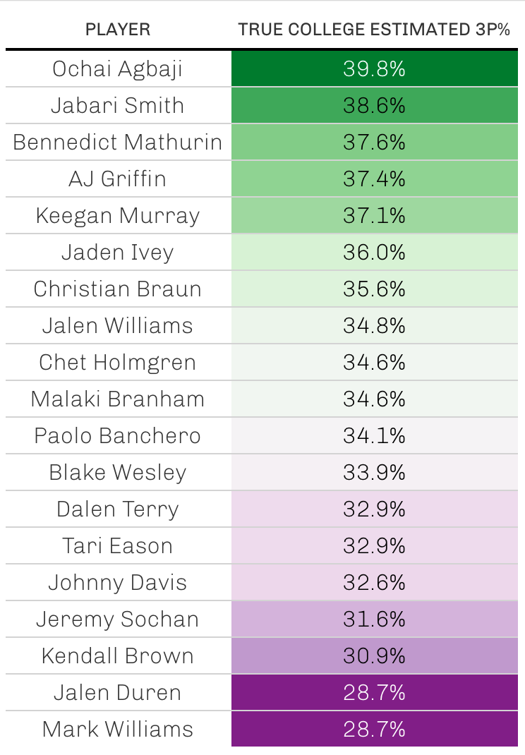
When applying this model to a variety of top projected picks for the 2022 draft, the following estimates were assigned for “true” college estimated three point percentage. The players who the model believes are the best shooters are at the top, with the worst at the bottom.

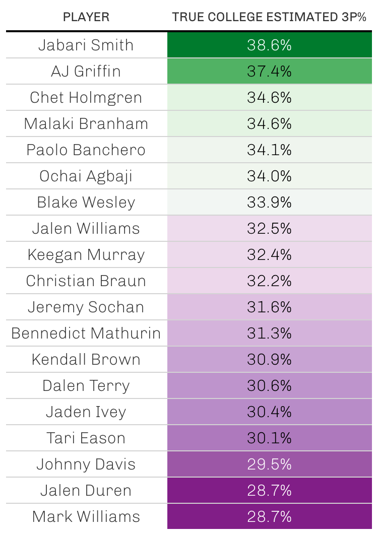
One other similar method involves iterating this process over multiple years, and whenever possible, using a player’s posterior distribution from their most recent season as their prior distribution for the upcoming season. This allows information about players to be carried across seasons.

Here are the results using this multiyear iterative model:

The nature of draft projections makes it necessary to publish them before the actual draft takes place, which is why I’m writing this post approximately 23 hours before the draft starts: to get them down on paper. In the future, I’ll return to this post and edit it to include a more thorough methodology, but here I’ve included the bare-bones outline and — most importantly — the complete results.